Particle-Mesh Force Calculator
Particle-Mesh in version 3.0 of Particle Physics Simulator
Particle-mesh in PPS 3.0
The new version 3.0 of the Particle Physics Simulator has been out for almost a month now, but I just had no time to write a post about it. I guess most of you already got the automatic update via the Android Market. The most notorious feature added is the incorporation of a new force calculator method which is selectable from the preferences screen. The force calculator method is the first of two steps in any simplified n-body code, where forces acting on each particle are calculated. Then, the integrator comes in to derive new accelerations, velocities and, ultimately, positions, which are conveniently updated and displayed in screen to create the illusion of a smooth animation.
In the basic direct method each particle’s force is calculated directly applying Newton’s second law of motion, where given initial positions \(q_i\) and velocities \(\dot q_i\) for the \(i\) particles, we can get the forces with:
$$f_i = m_i \ddot q_i = G \sum \frac{m_j m_k (q_k - q_j)}{|q_k q_j|^3}~ j = 1,\cdots,n$$
where \(n\) is the number of particles and \(q_i\), \(\dot q_i\) and \(\ddot q_i\) are their positions, velocities and accelerations. The complexity of this method is \(\sim O(n^2)\).
Now, the new Particle-Mesh (PM) force calculator method uses a whole different approach.
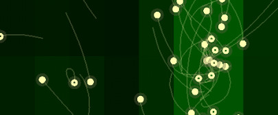
Particle-mesh method in the app. The background colors represent the grid weights.
The simulation are is divided into zones using a static grid, whose vertices are assigned at each time step a density value using the cloud-in-cell method, where particles are modeled as density areas whose contribution to a vertex depends on the particle’s area inside the vertex’s influence region. Once we have a density function, create a bicubic spline 3D surface so that potential wells are actually represented by craters, and low-potential zones are represented by humps. In a serious code, one should go from density to potential energy using Poisson’s equation (FFT), but we adopted a fastest albeit physically inaccurate approach. This PM method reduces the computational complexity of the problem to \(\sim O(n + n_g \cdot log n_g)\) where \(n_g\) is the number of vertices in the grid.
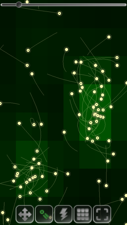
Finally, there’s an option in the app to display the grid densities as a colour map. What it’s doing is selecting a series of points in the 3D surface and get its height. Zones where the green colour is saturated indicate potential wells, and blackish zones indicate humps. I’ll shortly post a full description of my naive implementation of the PM method for the Particle Physics Simulator.
As usually, you can get the update from the Android Market.