Sparse Virtual Textures
A technical description of my implementation of Sparse Virtual Textures in Gaia Sky
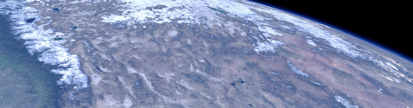
Real time rendering of the Earth in Gaia Sky with surface, cloud and height virtual textures.
Implementing proper virtual texture support in Gaia Sky has been on my to-do list for many years. And for many years I have feared that very item, as the virtual texture mechanism is notoriously complex and hard to implement. However, once working, they are very cool and bring a lot of value to software like Gaia Sky. In this post, I describe and discuss my implementation of virtual textures in Gaia Sky in detail, and provide a thorough examination of some of its most interesting points. If you are looking for the specifics of how to define or use virtual texture datasets in Gaia Sky, please refer to the official documentation. Here I provide only a general technical description.
Overview
Virtual Textures (VT), also known as Sparse Virtual Textures (SVT), MegaTextures1, and Partially Resident Textures (PRT)2, have at their core the idea of splitting large textures into several tiles and only streaming the necessary ones (i.e. the ones required to render the current view) to graphics memory in order to optimize memory usage and enable the display of textures so large that they can’t be handled effectively by the graphics hardware.
This technique aims at drastically increasing the size of usable textures in real time rendering applications by splitting them up in tiles and streaming only the necessary ones to graphics memory. It was initially described in a primitive form by Chris Hall in 19993 and has subsequently been improved upon. My understanding is that most modern implementations are based on Sean Barret’s GDC 2008 talk on the topic4.
In this article we use VT and SVT interchangeably to refer to virtual textures.
How Do They Work?
Virtual texturing is the CG memory counterpart to the operating system virtual memory. In virtual memory, a process’ memory address space is divided into pages, which are moved in and out of a cache space depending on whether and when they are needed. In virtual texturing, textures (images) are split up into smaller tiles and paged in and out of a cache texture when needed.
Virtual texturing requires some pre-processing to be done, as the large texture needs to be split up into tiles beforehand. The tiles in our implementation need to have a 1:1 aspect ratio (i.e. must be square). There are four main steps in every virtual texture implementation:
- Tile determination – first, we need to determine what are the visible tiles in our scene, with the current camera position, orientation and field of view.
- Cache – then, we use the information in the first step to fetch the observed tiles and put them into a cache texture, that we’ll send to graphics memory.
- Indirection – after that, we update an indirection (lookup) table with the location of the tile in the cache, and also send it to graphics memory.
- Rendering – finally, we can use the cache and indirection textures to render our scene with a special fragment shader that converts virtual texture coordinates to physical texture coordinates.
Tile Visibility
First of all, we need to know what are the visible tiles at every moment. We can determine the observed tiles by rendering the scene to an off-screen frame buffer with a special shader that computes the tile we need for each fragment. Since we are only interested in the tile information, we can get away with rendering this pass to a downsized frame buffer. In our implementation, the tile determination frame buffer is 4 times smaller than the main render buffer in width and height (16 times smaller in area). This factor will be important later.
A first approach might be just outputting the \((x,y)\) coordinates of the tile (column and row, if you will), together with the tile ID. We compute the coordinates by multiplying the texture coordinates (in UV) by the SVT dimension in tiles, and floor the result to have whole integers. In the following code we put the tile coordinates in the red and green channels, and the SVT ID in the blue channel.
uniform float u_svtId;
uniform vec2 u_svtDimensionInTiles;

in vec2 texCoords;

out vec4 fragColor;

void main() {
  fragColor.xy = floor(texCoords * u_svtDimensionInTiles);
  fragColor.z = u_svtId;
}
The tile determination pass frame buffer of the Earth with a virtual texture with 2048 (64x32, with a 2:1 virtual texture) tiles.
The image above shows the tile detection frame buffer (with channels scaled for visibility) for a virtual texture with 2048 tiles (64 tiles in width times 32 tiles in height). This approach has some issues:
- No matter how near to or far from each fragment we are, we always end up hitting the same tile. Remember that so far, tiles have a fixed resolution and cover a fixed area.
- Since tiles are loaded on demand, when a tile is not yet available in the cache the system won’t know what to render and leave a blank space, producing visual artifacts.
The solution to both these problems is introducing levels of detail. In textures, levels of detail are implemented through mipmaps.
Good to know
Mipmaps, also called MIP maps or pyramids, are pre-computed sequences of images that are successively lower-resolution versions of the previous. MIP is an acronym that stands for the Latin multum in parvo, meaning ‘much in little’.
Mipmapping
We modify our original formulation, and instead of dividing the texture into only a bunch of tiles that all cover the same area, we generate a tree, with the whole texture at the root. Each level contains 4 times the amount of tiles of the level directly above, and each tile covers 4 times less area. The resolution of all tiles in all levels is still the same though. We have a quadtree!
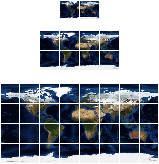
An example of a virtual texture with 3 levels (0 to 2) for the Earth laid out as a quadtree. Note that the root (level 0, top), covers the whole area, while successive levels have equally-sized tiles that cover less and less area each. This VT has an aspect ratio of 2:1, so it has two root nodes at the top.
In our quadtree, level 0 contains one or two tiles (depending on SVT aspect ratio) which cover the whole area (left tile in the image), and the level numbers for each tile indicate its depth. In the image, pictured top to bottom are levels 0, 1, 2 and 3.
Note
Mip levels and quadtree levels are not the same! In our tree, the level 0 is the root, which contains the lowest-resoltuion tiles. In mipmaps, mip level 0 is the base level, containing the texture at its full resolution!
If we incorporate the quadtree with different levels, the shader we showed before gets a bit more complicated. First of all, we need to determine the LOD level of the fragment. To do so, we could use the GLSL function textureQueryLod(sampler2D s, vec2 texCoords), but we’d need a texture bound in that fragment shader, which we do not have. However, that function can be easily implemented with some partial derivatives,
$$\begin{eqnarray} D_x &=& \left(\frac{\partial u}{\partial x}, \frac{\partial v}{\partial x}\right), \\\ D_y &=& \left(\frac{\partial u}{\partial y}, \frac{\partial v}{\partial y}\right), \\\\ L &=& log_2(max(|D_x|, |D_y|)), \end{eqnarray}$$
where \(u\) and \(v\) are the UV texture coordinates, and \(x\) and \(y\) are the window x and y coordinates. We can use dFdx() and dFdy(), which do precisely that, to get the mip level:
float mipmapLevel(in vec2 texelCoord, in float bias) {
    vec2  dxVtc        = dFdx(texelCoord);
    vec2  dyVtc        = dFdy(texelCoord);
    float deltaMaxSqr  = max(dot(dxVtc, dxVtc), dot(dyVtc, dyVtc));
    return               0.5 * log2(deltaMaxSqr) + bias;
}
And then, we can implement the tile detection like this:
uniform float u_svtId;
uniform float u_svtDepth;
uniform vec2 u_svtResolution;

in vec2 texCoords;

out vec4 fragColor;

// Scale factor of our tile detection frame buffer w.r.t. the window.
const float svtDetectionScaleFactor = -log2(4.0);

void main() {
    // Aspect ratio of virtual texture.
    vec2 ar = vec2(u_svtResolution.x / u_svtResolution.y, 1.0);

    // Get mip LOD level.
    float mip = clamp(floor(mipmapLevel(texCoords * u_svtResolution, svtDetectionScaleFactor)), 0.0, u_svtDepth);
    // In our tree, level 0 is the root.
    float svtLevel = u_svtDepth - mip;
    fragColor.w = svtLevel;

    // Compute tile [x,y] at the current level. Can also be seen as the column and row.
    float nTilesLevel = pow(2.0, svtLevel);
    vec2 nTilesDimension =  ar * nTilesLevel;
    fragColor.xy = floor(texCoords * nTilesDimension);

    // ID.
    fragColor.z = u_svtId;
}
There are a few things to unpack here:
- The mip LOD level 0 is the base level with the highest resolution. This is reversed in our quadtree, where the level 0 is the root with the lowest pixel/unit area ratio. That is why we convert from mip level to SVT level using the tree depth.
- The
u_svtResolutioncontains the base resolution of the SVT, i.e., the resolution of the deepest level. nTilesDimensioncontains the size of the level in tiles.- Here, we put the tile coordinates in the red and green channels, the SVT ID in the blue channel and the level in the alpha channel.
- Finally, when we are getting the mip level in the shader, we do so using the window \((x,y)\) coordinates in the tiny, scaled-down frame buffer. We need to apply a factor to get back the real mip level in our main window! The
svnDetectionScaleFactoris precisely that, and is computed from the frame buffer reduction factor with respect to the window (that factor is 4 in our case). The area of a frame buffer scales with the square of the sides, so we use \(log_2()\). The factor is negative because we need to move to more detailed levels (closer to 0 in the mip LOD level scale) when rendering to a larger frame buffer.

The tile determination pass frame buffer, with values scaled for visibility, using mip levels. The different levels show as rings on the Earth, starting with level 0 (outermost ring, darker), down to level 4 (innermost ring, brighter).
Frame Buffer Format
We use a frame buffer with a depth attachment and a floating point texture attachment with 32 bits per channel. This allows for \(~2^{32}\) values per channel, which provides ample precision to accommodate trees with up to 31 levels. To put this in perspective, if we map the Earth with a tree with 31 levels, each tile covers ~1cm. Any tile resolution greater than 100x100 provides sub-millimeter precision on the whole planet.
Note that, in order to be able to read back the pixels cleanly, we need to enable the depth test and disable alpha blending, especially if we have concave objects or we support more than one SVT.
Tile Cache
Once we have rendered the tile detection frame buffer, we can read it back to main memory with glGetTexImage() (remember to use the right format and type). With that, we obtain a list of the observed tiles in the CPU, where each entry has the tile ID, the level, and the column and row in that level. The observed tiles are then loaded from disk asynchronously, and when they are ready, they are added to the tile cache.
The tile cache itself is just a texture whose size is a multiple of the tile size. Since we only support power of two tile sizes in the range \([4, 1024]\), our tile size is always a multiple of 1024. Currently, our implementation sits at 1024*12, so that the tile cache can fit 12x12 tiles of 1024x1024 resolution, or four times that number of tiles at 512x512 resolution. This ensures that the tile cache size is always divisible by the tile size.
When tiles are added to the tile cache, they are put in the first empty space available. If we don’t have empty spaces, an LRU (least-recently used) strategy is used, where the tile that has been visited least-recently goes out. Level-0 (root) tiles never go out, and always stay in the cache. We’ll come back to that later.
In order to actually add a tile to the cache we use glTexSubImage2D(target, level, x, y, w, h, format, type, buff) to draw on the texture at a specific mip level, and a specific position. The size (w and h) is always the same, which is the tile size. In OpenGL, context calls need to happen synchronously in the context thread (unlike Vulkan), so when tiles finish loading asynchronously, the main thread picks them up and writes them to the cache.
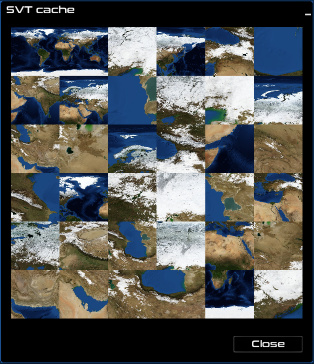
Gaia Sky can visualize the contents of the tile cache in real time. In the image, a tile cache of 6x6 tiles (the texture has a resolution of 6144x6144, as the tiles are 1024x1024). Note that the two root tiles covering the whole Earth are located to the top left of the cache. These tiles never move!
But still we are not done. What do we do with the cache? How do we find out in the texturing shader the actual location of the tile we need in the cache? Welcome to the wonderful world of the indirection table.
Indirection Table
In virtual memory, a table (often called pagetable) is used to translate from virtual memory addresses to physical memory addresses. This pagetable contains the physical location of each memory page indexed by virtual address.
In virtual texturing we use exactly the same concept. We will generically call it indirection table, but we’ll actually materialize it with another texture, of course!
Fun fact
In graphics programming, textures are really versatile. They are most commonly used to store image data, but they can also be used to store any kind of data required! In GPGPU, 1D, 2D and 3D textures are used all the time to store datasets and scientific data.
Since our virtual texture is kind of mipmapped (different levels provide different resolutions, which are accessed depending on pixel gradients), our indirection table is also mipmapped. Also, the indirection texture must provide a means to translate from virtual texture coordinates (UV, the ones we get in the fragment shader) to physical texture coordinates in the cache. This means that we need one pixel per tile, so our indirection texture for an SVT with 3 levels (0, 1 and 2) will be a mipmapped 4x4 texture, as the deepest level, 2, has \(2^2=4\) tiles per side.
In OpenGL, remember to set the correct minification filtering so that mipmaps are actually used. We don’t use trilinear filtering, so we set the minification filter strategy to GL_NEAREST_MIPMAP_NEAREST. The magnification filter is set to GL_NEAREST, as we don’t want interpolation to pollute our values.
But how do we fill the indirection texture? Each pixel represents a single tile. For each pixel we store the tile \((x,y)\) coordinates in the tile cache, plus the actual tile level. Additionally, we use the alpha channel to store the validity. A value of 0 means that the tile is not valid (removed or not yet set), while a value of 1 means the tile is valid. With this, we can remove tiles by just setting their alpha value to 0.
Each RGBA pixel in the indirection buffer contains:
- R – tile X location in the cache (column).
- G – tile Y location in the cache (row).
- B – level.
- A – validity (0=invalid, 1=valid).
Let’s see a practical example in the following figure:
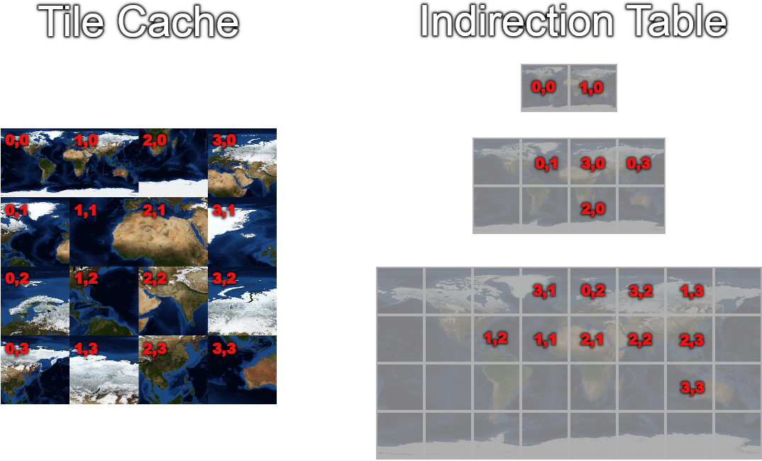
An image showing the tile cache with 4x4 tiles (left), and the indirection table for this particular configuration of the tile cache (right). The SVT has three levels and is shown in the mipmapping section of this post.
The SVT corresponding to this figure is shown in this other figure. Note that the indirection table has three mip levels, like the SVT, but in this case these are actual mipmap levels. Each ‘box’ in each level is only one pixel in the indirection texture! As you can see, the contents of each pixel refer to the positions of tiles in the cache. Some pixels are empty. This means that their tiles are not in the cache. In that case, we mark them with alpha=0.
Since each pixel only needs to hold the coordinates in the tile cache and the level, which are usually low numbers, we can get away with a format using less bits per channel this time around, so we use a float bufferr with 16 bits per channel, GL_RGBA16F.
Now, there are two strategies as to how to proceed.
- First, we can decide to complete pixels in lower levels in the indirection table with references to tiles in higher levels that cover the same area. This is elegant, as it ensures that we always have a fallback plan, and it allows us to just query the specific level in the fragment shader, but it involves some additional processing in the CPU side to fill in the empty bits in the indirection texture.
- The second option is leaving the table with ’empty’ pixels and loop in the fragment shader from the desired level up in the mipmap sequence. This also makes sure that we always have a fallback tile to default to (remember level 0 tiles are always in the cache), but it involves some additional looping and texture lookups in the fragment shader. The number of iterations and lookups is, in the worst case, the number of levels of the SVT.
In our implementation, we use the second option, as we find it easier to understand and implement. Performance-wise, we have not compared it to the first option, but we would not expect a significant impact.
We are finally ready to write our texturing shader and experience all that high-resolution texturing goodness! Yay!
Texturing Shader
The final piece of the puzzle is using the indirection table in the fragment shader to transform virtual texture coordinates to coordinates in the tile cache. Since we have empty pixels in the indirection table, we also need to implement the iterative texture lookups to the different mip levels. Here is the code:
/*
This function queries the indirection buffer with the given texture coordinates
and bias. If the tile is invalid, it sequentially loops through the upper levels
until a valid tile is found. The root level is always guaranteed to be found.
*/
vec4 queryIndirectionBuffer(sampler2D indirection, vec2 texCoords, float bias) {
    float lod = clamp(floor(mipmapLevel(texCoords * u_svtResolution, bias)), 0.0, u_svtDepth);
    vec4 indirectionEntry = textureLod(indirection, texCoords, lod);
    while (indirectionEntry.a != 1.0 && lod < u_svtDepth) {
        // Go one level up in the mipmap sequence.
        lod = lod + 1.0;
        // Query again.
        indirectionEntry = textureLod(indirection, texCoords, lod);
    }
    return indirectionEntry;
}

/*
This function converts regular texture coordinates
to texture coordinates in the SVT buffer texture
using the indirection texture.
*/
vec2 svtTexCoords(sampler2D indirection, vec2 texCoords, float bias) {
    // Size of the buffer texture, in tiles.
    float cacheSizeInTiles = textureSize(u_svtCacheTexture, 0).x / u_svtTileSize;

    vec4 indirectionEntry = queryIndirectionBuffer(indirection, texCoords, bias);
    vec2 pageCoord = indirectionEntry.rg;// red-green has the XY coordinates of the tile in the cache texture.
    float reverseMipmapLevel = indirectionEntry.b;// blue channel has the reverse mipmap-level.
    float mipExp = exp2(reverseMipmapLevel);
    // Need to account for the aspect ratio of our virtual texture (2:1).
    vec2 withinTileCoord = fract(texCoords * mipExp * vec2(2.0, 1.0));
    return ((pageCoord + withinTileCoord) / cacheSizeInTiles);
}
This code should be quite self-explanatory, as it is heavily commented. If we did not support non-square virtual textures it could be simplified. The queryIndirectionBuffer() method does the indirection texture lookup at the level determined by the method mipmapLevel() (we have seen it before), and loops down the mip levels until a valid tile is found.
Filtering
However, when we inspect the results, we find seams! This is due to the use of bilinear texture filtering. You see, texture filtering uses samples from adjacent texels to interpolate the color, which makes sense in regular textures, but when sampling from our tile cache texture, unrelated tiles sit next to each other, leading to the usage of totally unrelated texels from adjacent tiles to perform the filtering.
Seams are visible in the boundaries between tiles due to bilinear filtering in the tile cache texture, where tiles from different areas sit side-by-side.
There are two possible solutions to this:
- We just don’t use linear filtering, and default to nearest-neighbour. This is unacceptable, especially in magnification, which displays the textures pixelated with clear boundaries between texels.
- We prepare our tiles so that they include a 1-pixel border with the contents from adjacent tiles. This reduces the usable tile resolution from \(N\times N\) to \(N-2\times N-2\) (2 for left-right and top-bottom borders). We have to take this into account in our texturing shader when determining the within-tile coordinate, i.e., the coordinate of the texel we need to query in the tile, by updating its value using the tile size,
$$ c = \frac{c_{xy} * s * 2}{s} + \frac{1}{s}, $$
where \(c_{xy}\) is the within-tile coordinate, and \(s\) is the tile size.
We need to add the following line in our svtTexCoords() method, right before the return statement:
// The next line prevents bilinear filtering artifacts due to unrelated tiles
// being side-by-side in the cache.
// For each tile, we sample an area (tile_resolution - 2)^2, leaving a 1-px border
// which should be filled with data from the adjacent tiles.
withinTileCoord = ((withinTileCoord * (u_svtTileSize - 2.0)) / u_svtTileSize)
                  + (1.0 / u_svtTileSize);

Seams are gone!
Here are some videos of the system working at full strength, with different channels per object and multiple SVTs.
Exploring South America.
The south of the UK using an SVT with 10 levels.
The Earth using a surface and an elevation SVT. The elevation SVT is queried in the tessellation evaluation shader to determine the elevation at each tessellated vertex and modify its height accordingly.
Tools
We did not find any open-source tools to our liking to create virtual textures from high-resolution texture data, so we created our own. You can find them in the virtual texture tools repository. This repository contains two scripts:
split-tiles— can split a texture into square tiles of a given resolution, and names the tiles in the format expected by Gaia Sky (and also Celestia), which istx_[col]_[row].ext. The output format, quality and starting column and row are configurable via arguments.generate-lod— given a bunch of tiles and a level number, this script generates all the upper levels by stitching and resizing tiles. It lays them out in directories with the formatlevelN, where N is the zer-based level. The input tiles are also expected in a directory. The output format and quality are configurable.
Additional Considerations
In our implementation, we had to consider some additional issues:
- We need multiple SVTs per object for the different maps (diffuse, specular, normal, elevation, emissive, metallic, roughness, clouds). The IDs are unique per object (all SVTs of the same object share the same ID), so that the tile determination pass works for all channels, but every SVT has its own indirection table.
- We had to adapt the tessellation shaders to query the SVT for height data. This lookup is not made in the fragment shader, but in the tessellation evaluation shader, so
dFdx(),dFdy()andtextureQueryLod()are not available.
Limitations
The limitations of our implementation are the following:
- Due to the fact that all SVTs in the scene share the same cache, right now we can’t have SVTs with different tile sizes in the same scene.
- Similarly, only square tiles are supported. Actually, we can’t think of a single good use case for non-square tiles.
- Supported virtual texture aspect ratios are \(n:1\), with \(n\geq1\). This is due to the fact that VT quadtrees are square by definition (\(1:1\)), and we have an array of root quadtree nodes that stack horizontally in the tree object. It is currently not possible to have a VT with a greater height than width.
- Performance is not very good, especially with many SVTs running at once. This may be due to the shader mimpmap level lookups. This produces \(depth\) texture lookups (mip levels) in the worst-case scenario when only the root node is available in the cache. A workaround would be to fill lower levels, additionally to the tile level, in the indirection buffer whenever a tile enters the cache. This would also have a (CPU) overhead. Might be faster.
- All SVTs in the scene share the same tile detection pass. This means that there is only one render operation in that pass. This might be good or bad, I’m not quite sure yet.
More
If you want to read more on the topic or expand on what is described here, I suggest the following resources.
- Albert Julian Mayer’s master thesis on the topic is a very good academic resource which thoroughly describes the technique and discusses several topics in detail. I have used it as a valuable resource during the implementation.
- OpenGL defines
ARB_sparse_texture5, a vendor-agnostic extension for virtual texturing. I have not used it in this implementation, but probably could. It is based on an original extension by AMD,AMD_sparse_texture6. Here is a nice comparison.
Hall, C. — Virtual Textures: Texture Management in Silicon [pdf]. ↩︎
ARB_sparse_textureextension documentation. ↩︎AMD_sparse_textureextension documentation. ↩︎